 |
 |
 |
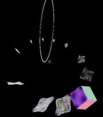
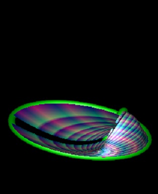
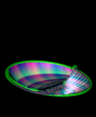
| Any CAD gesture taking a line rotation axis or a uniform displacement extrusion has a well defined mathematical generalisation easily user interfaced simply by replacing the linear axis or displacement vector control with a user circle input capable of handling the degenerate line and infinite-radius translation cases | If a is dual to a weighted sum of circles and lines, we have rotation "around" a "composite axies". Such rotations tend in general not to be closed or periodic, and may converge or diverge, but they are infinitaely smooth and differentiable analytically as a geometric product. Here a circular profile curve rotated ("swept") around a composite axis comprising weighted combination of two orthogonally, and nonorthogonally aligned circles. Any weighted combination of circles and lines canonically decomposes most generally into, in 3D, two mutually inversive (each it's own reflection in the other) real and imaginary circles whose commuting blade representations provide an easy factoring of the exponentiation into seperate simple trigonometric and hyperboolic computations. | |
The "canonical axies" for the circular sweeps are not shown in the above images,
but would usefully form part of a CAD comnposite rotation UI.
Any two such commuting circles or lines also generate for each position p0 an orthogonal
parametrisation of a rapidly computable 2-curve
p(u,v) º
e(½uB1)
e(½vB2)
p0
e(-½vB2)
e(-½uB1)
containing p0=p(0,0),
degenate cases of which include cylinders and tori, with Dupin cyclide knots emerging when the blades are coprimally weighted
|  |
 |
 |
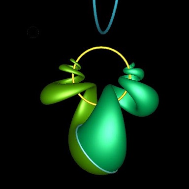
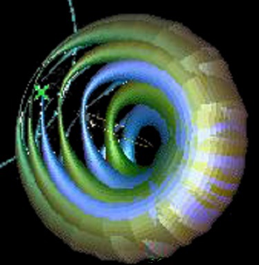
| Given two circles S1 and S2, the 2-vector logarithm of Â4,1 <0;2;4>-vector S2S1-1 provides interpolable transformation taking S1 to S2. One can rotate S1 to either S2 or -S2, giving two surfaces combining to enclose a naural BREP defined by the the two circles. | If the rotation is aperiodic, extending the S1 to S2 rotation over [0,1] to (-¥,+¥) provides a constant curl closed skin of the two circles. | ||
|  |
 |
|
|
The canonical decomposition of linear combinations of 3D circles into real and imaginary circles provides a more rapidly computable natural linear interpolation between cirlce. | Rotating a circular profile through a circular axis itself rotating through a circular axis produces a highly self intersective form. | ||
The general trajectory of points under rotation with a circular axis are circular but points on the straight axis axis traverse that axis.
The trajectortory of the origin e0 rotated in a circle of radius R centered on e0 with axis direction e3 is
cos(½q)2(e0 + tan(½q)Re3 + tan(½q)2R2e¥)
leaping from ¥e3 to
-¥e3 with zero weight as q passes through p, and decelerating to return to e0 at q=2p with speed R,
The angle required to translate (0,0,z1) to (0,0,z2) along the z-axis is
2( tan-1(R-1z2) - tan-1(R-1z1)).
If we localise a rotation through a single hoop of a surface element substantially parallel to the hoop,
or a composite axis dominated by such a hoop, we obtain a rotational extrusion emboss,
but generalising it it in four distinct and fundamental ways:
the sketch lines lie in a general surface rather than a plane;
the extrusion is a rotation around a composite axis rather than translation in a common z direction
(tending as the radius of an axis hoop approaches infinity to a unidirectional translational extrusion);
The extent of the extrusion is variable (localised) rather than uniform across the sketch; and
rather than driving and defining the edges of new surfaces,
the sketch lines extrude as ridges, folds, or bulges (depending on b)
in a shared surface.
Conformally embedded positions reside on the "null horosphere"
{ p : p2 = 0 ; p¿e0 = 1} .
To accomodate tolerance one embeds instead in a
tolerance horosphere
{ p : p2 = h2 ; p¿e0 = 1} for small real h
using
origin grain eh º e0 - ½h2e¥
with eh2 = h2 in place of e0 when corformally embedding positions.
We will refer to a sphere of radius close to h as a grain and a sphere of
radius precisely h as an exact grain.
Because GHC stores the (squared) radius of a sphere "mixed in" with the center coordinates,
the precision of the radius is merged with and comparable to the precisions of the coordinates,
exact grains cannot be represented except at exceptional positions; and
as we process a grain p through geometric computations, its radius may drift
further from h, with p2 - h2 providing a computable measure of
the imprecision of both radius and the positional coordinates.
The product ab of two distinct embedded positions a, b
is a scaler representing their seperation and a 2-blade aÙb
dual (in 3D) to an an imaginary circle once intersected with null horosphere.
For granular a and b,
if aÙb)2 £ 0
then the grains are close, intersecting in a circle (or a point if they are just kissing) when
aÙb dually embodies the "intersective pencil" space of all
spheres and planes whose surfaces contain that circle, which on restriction to the
tolerant horosphere gives the two exact grains that meet at the circle.
If a and b are large grains meeting in a circle of radius > h
then we have something imaginary in the tolerant horosphere instead, and the
two grains can be considered super-same,
even more the same grain than if they were the same grain, providing a computable "snap confidence".
If they intersect in a circle of radius precisely h then then their tolerant horosphere
outter product vanishes. We thus only lose all information from the outter product
of two distinct grains if they meet in a cicle of radius precisely h. This is computatonally less
likely than two singular positions being precisely the same, so grains preserve distinctness through equivalences better.
The product abc of three embedded positions a, b, and c,
has 3-blade component aÙbÙc representing the circle or line through the points,
and 1-vector component dual to the sphere passing through a and c with centre
(A2-B2+C2)-1 (Aa-Bb+Cc)
and radius -ABC(A2-B2+C2)-1 ;
where A is the distance between b and c etc.
When a,b, and c are grains rather than null positions
the coordinates of abc deviate slightly by order h2, the deviations
embodying helpful geometry.
If the three spheres intersect it is most generally in a bipoint
with aÙbÙc dually representintg the
3-bunch of all bipoints, lines, circles, planes and spheres contaning that bipoint.
Restricting the 3-bunch to to the tolerant horosphere gives all exact grains sat on by the bipoint,
sweeping a solid apple torus of minor radius h.
Given four sphere duals,
if they intersect the wedge provides an intersecting bunch of all k-sphers and k-planes sat on by the intersection.
If they do not intersect then aÙbÙcÙd is the "orthosphere" ,
the 2-sphere orthogonal to the four 2-spheres, dually representing the "Poncelet sphere" space of all spheres, circles, bipoints, planes etc. orthogonal to the orthosphere. Assuming the orthosphere has radius exceeding e, restricting to the tolerant horosphere gives a grainset sweeping a spherical "shell" of thickness e .
If the four spheres are far seperated grainst, the central sphere will differ from grain center spanned sphere
negligably at order h2 .
The wedge of four grains is a spherical h shell on their orthosphere.
The radius s of s* is such that the squared seperation from a to s*
plus that from b to s* equals the squared seperation from a to b.
The locus of
la + mb is
somewhat analagous to an ellipse with foci a and b, but moving through spherespace and adding signed squared lengths.
A sphere centred between a and b has to have imaginary radius to
allow the squared seperations to add correctly.
Only when l and m have opposite sign corresponding to an "averaged position" outside the line segment between a and b
can the sphere have a real radius.
Adding positions provides a natural "radius" for facets.
If we add K coplanar positions p1, p2, ..pK then their conformal
åi pi = K(e0 + (K-1)-1åi pi - (K-1)-1åi¹j (pi - pj)2)
is a K-weighted antisphere of radius (K-1)-1 (åi¹j (pi - pj)2)½
centered at the conventional facet "center".
If the facet is an equilateral triangle, this is the radius of the circumcircle.
For a reular polygon it is K-½ times the side length.
If the triangular facet is very flat and thin with lengths A » 2B»2C
this is approximately 6-½A.
If the facet is tall and thin with A»B and small C or a right-angled triangle with hypotenuse A
it is 2½A.
Let S=aÙbÙd be as circle through points a,b,d
and assume we are interested in the circular arc from a to b that excludes d. Let D be a sphere centred d
of radius D>0; typically we might hacve D=1 and D=(e0+d+½(d2-1)e¥)* .
Krasauskas observes that as S inverts in D into line
D(S) = DS(D#)-1 = D(a)ÙD(b)Ùe¥ so we can parameterise the arc from a to b
as the inversion in bl(D) of a linear interpoaltion from D(a) to D(b).
Taking u to the displacement vector projection of D(b)-D(a) into the unembedded pseudoscalar we have
a rational parameterisation D( (1+½te¥u)D(a)(1-½te¥u) )
of the circular arc from a to b.
Similarly a spherical patch (with circular arc boundary elements) inverts in any sphere centered on a point outside the patch on the sphere
to a planar patch (with planar circular arc boundary elements), and a Bezier curve on a sphere can be inverted to a rational planar curve ..
Dupin cyclides are of relevance to CAD both as natural blends between quadratic surfaces and as genertors of circular arc structures of freeform architecture.
A Dupin cyclide patch inverts in the cyclide's sphere of inversion to a conic, cyclindrical, or toroidal patch.
One natural GA representation of a Dupin cyclide is perhaps the three mutually tangental spheres
whose envelope of cotangential spheres defines the cyclide, however Dupin Cyclides can also be considered as circles in sphere space.
piKe337!3
pi
Dorst shows that the N+2 orthogonal eigenvectors of the symmetric linear mapping
P(x) = åi=1M pi(pi¿x)
correspond to N+1 orthogonal (intersecting at right angles) ordered real hypersheres and one orthogonal imaginary (r2<0)
hypersphere maximising E(s and providing a potent, intuitive, and beautiful "covariant conformal eigenstructure" geometric interpretation of
the centroid and covariance matrix of a point cloud.
The imaginary sphere is a localiser having centre the centroid and squared readius the negative variance.
Rimas Krasauskas.
"Unifying thoory of Pythagorean-normal surfaces"
(AGACSE 2015 Presentation)
R. Krasauskas and S.Zube.
"Bezier-like Parameterizations of Spheres ans Cyclides Using Geometric Algebra"
Sebti Foufou and Lionel Garnier , 2004
"Dupin Cyclide Blends between Quadratic surfaces for Shape Modelling"
Leo Dorst
"Approximate Least Squares Fitting of Hyperspahers and Hypercircles using CGA"
(AGACSE 2012 Presentation)
Pablo Colapinto
"Articulating Space: Geometric Algebra for Parametric Design Symmetry, Kinematics, and Curvature"
Localised Rotations
A localiser is a set of n geometric objects S1,S2,..Sn proximity to which we wish to measure.
We require a separation s(p,S) measuring the seperation of a given point p from object S that is 0 on
S and nonzero away from S, possibly signed according to inside/outsideness wrt S.
We use n pre-pulse Real() ® (-1,1) functions
z1,i(s)
with z1,i(0) small and tending to ±1 for large |s|, such as
z1,i(s)
=(1 + s2+ei)-1(s2+ei) mapping 0 to (1+ei)-1ei .
Having combined the separate separations s(p,Si) into a single bounded separation
from the localising set {Si} with the product
s(p, {Si}) = Pi=1n zi(s,p,Si)
one can use a final pulse function z2(s) mapping [-1,1] to [-M,M] with
z2(0)=M and
z2(±1)=0
to convert bounded separation s(p, {Si}) into a bounded proximity potential or#
agitation factor locally maximised on each mv(S)
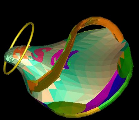
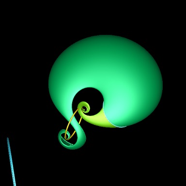
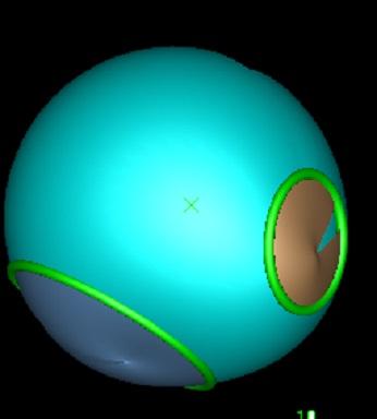
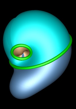
Rotation through a circular axiws, localised by proximity to that axis.
So it "bulges" the model through the hoop, providing an intuitive and controllable CAD gesture
for pulling and pushing models.
Quite late in the non-localised rotation through a cricular exis with axis passing through the model,
the lettered surface axis meet having passed through ¥ but the base of the "bowl" remaining to do so.
the model has inverted and is inside out
, a void in an infinite solid, which is why the lettering is reversed,
The handle of the basket is inside the void, so appears to be inside the BREP.
Because the rotation is not localised, no self intersections are introduced.
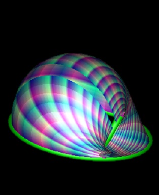
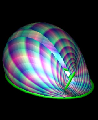
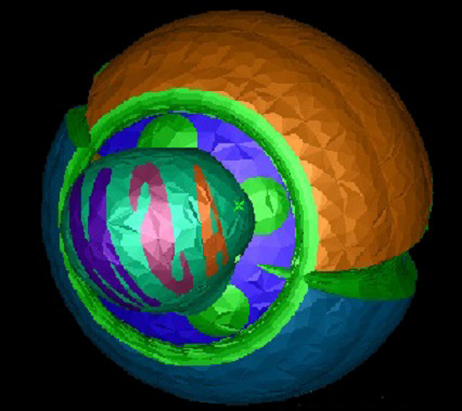
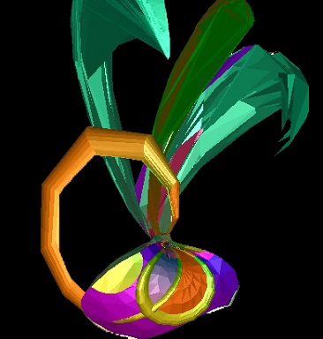
Here a rotation trhough a circular axis localised by proximity to another circle. Points rotated to outside an imposed
bounding sphere B are invereted in that bounding sphere p ® B*pB*,
introducing G1 discontinuities at the surface of the bounding sphere but converting the infinite discontinuities
at infinity to continuous traversal through its center, and potentially introducing self-intersections.
This is also quite late in the rotation, and there has been considerable reflection back into the bounding sphere,
resulting in "fronds". This deformation is specified by just two circles, a bounding sphere, three localising parameters and the
transform angle q.
Tolerant Positions
When computing geometrically we encounter computational noise and imprecison.
The same thing computed two different ways is unlikely to be recognised the same by == .
Typically, geometric programmers add a small positive positional "tolerance" h and decree
that any seperation less than it is zero, or at least ignorable.
In conformally embedded GA, 1-vector
s = s( e0 + c + ½(c2 - r2)e¥ )
is interpreted as dual to a (N-1)-sphere of center c and radius r, weighted by scalar s.
We have s2 = s2r2 and
allow "imaginary" or anti-spheres with r2 < 0.
The wieght s gives problems only when passing through or near zero which it usually
does only as c passes through infinity, often smoothing out
infinite dicontinuities as a BREP inverts.
When r=0 we have a position or point
p with p2 = 0, suggesting positions be viewed as dual to zero radius spherical sprfaces,
whose nullity makes their exponentiate trivially and the products of positions are particularly elegant and intuitive.
If aÙb)2 > 0
then the grains do not (dually) intersect and aÙb numerically embodies
particular positions p and q mutually inversive in both
a and b in that the reflection (inversion) of p in the a sphere is q ,
and the reflection of p in the b sphere is also q.
If the reflection of
p in another sphere, or plane, c is q then we will have
aÙbÙc = 0 .
Thus for non-intersecting a* and b*
the 2-blade aÙb dually embodies a "Poncelet pencil" space seperating the spheres.
In the more likely case of their not intersecting,
writing aÙbÙc = (ac - A2e¥)^(bc - B2e¥)^(ccc - C2e¥)
where ac,bc,cc are the embedded centers of the spheres,
aÙbÙc dually represents a
Poncelet circle of all k-planes and k-spheres orthogonal to the orthogonal
(aka radical) circle of the three great circles defined by intersecting the spheres
a*,b*, and c* with the plane
e¥ÙacÙbcÙcc .
The orthocircle represented conformally by aÙbÙc solves "Monge's Problem" and
the wedge product of three grains is an h torus on their orthocircle (aka. radical circle).
Adding Positions
Most geometry kernals fail to provide operator::+(position, position)
or operator*(double,position) because they mistakenly consider such geometrically meaningless.
More precisely: la + mb is only considered meaningful when
l=-m (a (scaled) displacement vector); or when l + m = 1
(a collinear point).
To make position-space a vector space
we recognise points as dual to zero radius spherical surfaces.
Setting a=e0 , b = e0 + xe1 + ½x2e¥ WLOG
we obtain
la + mb =
(l + m) (e0 + (l + m)-1m xe1 + (l+m)-1m½x2e¥)
which is the (l+m) weighted dual of the sphere with center
the averaged position (l+m)-1 (la + mb)
and squared radius
(l+m)-2lm(a - b)2
l+m is simply the weighting of the resultant sphere, it is the ratio
l:m that matters. If we rescale so that l+m=1 then the radius the sphere
la+mb is the geometric mean |lm|½
times the distance |a-b|, though if l and m have the same sign,
this is an antisphere. Thus the "midpoint" ½a+½b
is an antisphere of squared radius - ¼(a-b)2.
This is the radius that allows s¿a + s¿b
= (l+m)a¿b = - ½(a-b)2
and one can verify easily that
s¿a is ½(s2-(s-s)2)
which is just a particular measure of the separation between a and the surface of the sphere s*:
Typical of the sort of length measure provided by GA,
positive for a inside s* when it corresponds to the squared length of a
perpendicular to (a-s) from a to the sphere;
and negative for a outside s* when it corresponds to the squared length
of a tangent from a to the sphere.
Universal Geophysical Data Format
The 26=64 real coordinates of Â4,2n conformaly embedding Minkowski spacetime multivectors provide a generic
data packet for representing electromagnetic boosts, linear and angular momentae, 3D and spacetime spheres, circles, lines, planes, positions, vectoors,
and tangents, transforms, dilations, translations, quaternions, spinors , twists, shape and phyical tensors generally.
As Krasauskas observes, all three Laguerre geometry models are contained in Â4,2:
the cycolgraphic model in Â3,1, the Blaschke cylinder, and the Isotropic Model in Â2,0,1
with e¥ taypically taken as the null isotropic vertical.direction and e12 defining the "top view".
Adding a further spacial dimension
for the 128 coordinate conformally embedded Â5,1 provides a central i pseudoscalar and a simpler Dirac Equation.
e
Inversive Parameterisations
Whereas Geometric Algebra is not necessary for spherical inversion, particularly within the conformal embedding it provides
a natural and robust computational grammar for such and the manipulation of spheres and circles generally withinthe conformal embedding.
In Homogenous Coordinates, the inverse of p=p+e0 is
d+D2|p-d|-2 (p-d) + e0 =
d + (p-d)-1 , and the linear interpolation is
(1-t)(a-d)-1 + t(b-d)-1 + d) inverting to
(aw0(1-t) + bw1t) (w0(1-t) + w1t)-1
where w0 = (a-d)-1 , w1 = (b-d)-1 can be regarded as controll-point dependent
multivector weights of a generalsed rational Bezier curve. Such multivector weighted Bezier like curves are of increasing interest.
The 3-blade s1Ùs2Ùs3 represnts the Pencil
Pointcloud Analysis
Following Dorst, given a set of M conformally embedded N-D points pi we seek a best fit (N-1)-sphere
s* having centre c and squared radius r2 minimising "GA squared deviation"
E(s) = åi=1M s-2 (pi¿s)
= åi=1M r-2 (r2 - (c - pi)2)2)
= åi=1M di2(1 + r-1di + (½r-1di)2)
where di is the signed distance from pi to s*,
rather than the more usual (but recently questioned as biased) least squares fit sphere minimising åi=1M di2 .
Any locally minimising s solves (åi=1M pi(pi¿s)) Ù s = 0 and so is an eigemvetor of
P(x) = åi=1M pi(pi¿x) and since s¿P(s) = s2 E(s) we have E(s) = s-1¿P(s)
so the cost E(S) of a P() eigenvector s is the associated eigenvalue, so we seek the minimal nonnegative eigenvalue;
a standard linear algebra eigenvalue problem solvable faster than standard true least squares iterative aproaches.
The best fit (N-2)-spheres (hypercircles) are the ½N(N-1) eigenvectors of 2-blade "inertia" operator
P(s) = åi=1M piÙ(pi¿s), but are more readily available
as the intersections of the best fit hypershpheres, with best fit (N-3)-spheres being similar provided by intersctions.
The best fit hyperplanes and hyperlines under the GA squared deviation can also be cast as
an eigenproblem.
Referances/Source material for Multivector CAD Applications
http://uosis.mif.vu.lt/~rimask/old/pdf/Bezier-like.pdf
http://le2i.cnrs.fr/IMG/publications/918_09_eurographics2004-JointureQuadriques_CD4_dvd.pdf
http://portail-video.univ-lr.fr/Approximate-Least-Squares-Fitting
http://mat.ucsb.edu/pablo/dl/Colapinto_P_Dissertation.pdf
Glossary
Contents
Author
Copyright (c) Ian C G Bell 2015, 2016
Web Source: www.iancgbell.clara.net/maths
Latest Edit: 30 Jul 2016.